Jupyter Notebook¶

interactive computing
cells can be a code, markdown or raw text
prints out last time of cell, no need to add print()
use markdown to write your thoughts
two modes: command mode and edit mode

shortcuts to remember:¶

enter or double-click, start edit mode
esc to return to command mode
shift+enter execute current cell and move to next
ctrl+enter execute current cell and stay there
a and b, add cell above or below
dd delete a cell
c and then v, copy and paste a cell
m turn cell into markdown
y trun cell into code

The basics¶

# no data type declaration
a = 3
b = 19
a+b

# string concat
first_name = 'Shaji'
second_name = 'P'
first_name+' '+second_name

'Shaji P'

# string method example
statement = "this is a sentence"
statement.count('s')

# string method example
statement.split()

['this', 'is', 'a', 'sentence']

# Python list
x = [12,9,6,4]
y = [1,2,4]
x+y # lists are concatenated

[12, 9, 6, 4, 1, 2, 4]

# list method example
z = x+y
z.count(4)

# in-build sum function
sum(x)

# in-built sort
sorted(x)

[4, 6, 9, 12]

# using functions from math
from math import pi,sqrt
r = 4
sqrt(2*pi*r)

5.0132565492620005

Plotting¶

import matplotlib.pyplot as plt
import numpy as np # see next section
%matplotlib inline

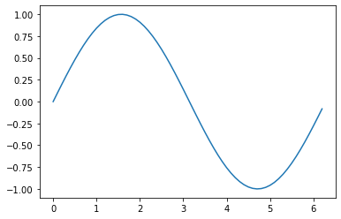
# create range of values from 0 to 2pi in steps of 0.1
x = np.arange(0,2*pi,0.1)

# create y as sine function with x as independent variable
y = np.sin(x)

# graph for the function y
plt.plot(x,y)

[<matplotlib.lines.Line2D at 0x7f1d0d5e3f70>]

Numpy¶

# numpy, the backborne of scientific computing 
# all array related operations are defined in numpy
import numpy as np

# create 2x3 array of 1's
x_arr = np.ones((2,3))
x_arr

array([[1., 1., 1.],
       [1., 1., 1.]])

# adds a scalar value element wise
x_arr + 4

array([[5., 5., 5.],
       [5., 5., 5.]])

x_arr
# to reflect change, store the values to the old array
# uncomment below two lines to see the change
#x_arr = x_arr+4
#x_arr

array([[1., 1., 1.],
       [1., 1., 1.]])

y_arr = np.array([2,2,2])
y_arr

array([2, 2, 2])

# array broadcasting
# matches the shape and adds the y_arr row to each -
# row of x_arr
x_arr + y_arr

array([[3., 3., 3.],
       [3., 3., 3.]])

y_arr = np.array([5,8])
x_arr+y_arr # broadcasting fails

---------------------------------------------------------------------------
ValueError                                Traceback (most recent call last)
<ipython-input-20-57fdba28a423> in <module>
      1 y_arr = np.array([5,8])
----> 2 x_arr+y_arr # broadcasting fails

ValueError: operands could not be broadcast together with shapes (2,3) (2,) 

# to rectifyabove error and add elements of y_arr to each column of x_arr
# change "orentation of y_arr" first
y_arr[:,np.newaxis] 

array([[5],
       [8]])

# now you can add them
y_arr[:,np.newaxis]  + x_arr

array([[6., 6., 6.],
       [9., 9., 9.]])

Speeding up operations with code change¶

import random
import numba

# create a list of 10k random elements
x = [random.random() for i in range(10000)]
y = [random.random() for i in range(10000)]
z = [] # empty list to store result

%%time
# first, let's try good old for loop
for i in range(len(x)):
    z.append(x[i] + y[i])
print(z[:3]) # print first 3 elements

[1.1532859016438493, 1.334577514000911, 0.3511312253827581]
CPU times: user 1.14 ms, sys: 416 µs, total: 1.56 ms
Wall time: 1.56 ms

%%time
# now list comprehension
z  = [x[i] + y[i] for i in range(len(x))]

CPU times: user 927 µs, sys: 0 ns, total: 927 µs
Wall time: 931 µs

%%time
# using zip()
# zip() and enumerate() are useful functions
z  = [a + b for a,b in zip(x,y)]

CPU times: user 747 µs, sys: 271 µs, total: 1.02 ms
Wall time: 1.02 ms

# create numpy arrays
xa = np.array(x)
ya = np.array(y)

%%time
# using numpy addition
za = xa+ya
za[:3]

CPU times: user 67 µs, sys: 25 µs, total: 92 µs
Wall time: 94.7 µs

array([1.1532859 , 1.33457751, 0.35113123])

# Take another example of finding sum of all elements in an array
# Below function finds sum of all elements in x
def add(x):
    total = 0
    for i in range(x.shape[0]):
        total = total+x[i]
    return total

# array of 10 million items
x = np.random.rand(10000000)

%%time 
add(x)

CPU times: user 2.04 s, sys: 0 ns, total: 2.04 s
Wall time: 2.04 s

4998375.354010175

Just in time (JIT) compiler¶

@numba.jit
def add_jit(x):
    total = 0
    for i in range(x.shape[0]):
        total = total+x[i]
    return total

%%time
add_jit(x)

CPU times: user 175 ms, sys: 524 µs, total: 176 ms
Wall time: 175 ms

4998375.354010175

%%time
add_jit(x) # already compiled, hence faster this time

CPU times: user 11.9 ms, sys: 214 µs, total: 12.1 ms
Wall time: 12.2 ms

4998375.354010175

%%time
# numpy sum
x.sum()

CPU times: user 5.6 ms, sys: 0 ns, total: 5.6 ms
Wall time: 5.04 ms

4998375.354010154

Remarks:¶

Python is not slow per say
the way you code matters
stick to existing fuctions in numpy when available
numpy functions are optimized for speed

Further references¶

example notebook
https://ipython-books.github.io/
learn more about matplotlib plots
https://github.com/fangohr/introduction-to-python-for-computational-science-and-engineering

Aim Text files and CSV

Oceanography with python

Jupyter Notebook¶

shortcuts to remember:¶

The basics¶

Plotting¶

Numpy¶

Speeding up operations with code change¶

Just in time (JIT) compiler¶

Remarks:¶

Further references¶